Remote Sensing Lab 7: Photogrammetry

Goal
The primary goal of this lab is to become more familiar with performing photogrammetric tasks on aerial photographs and satellite images. This involved calculating photographic scales, measuring areas and perimeters of features, and calculating relief displacement. In addition, it also introduces stereoscopy and performing orthorectification on satellite images. After going through this lab, I will have an understanding of photogrammetric methods performed on photographs and satellite images.

Methods
The first task is calculating the scale of a nearly vertical aerial image shown in Figure 1. To find the scale we need to use the equation that compares the size of real world features to the image. The equation is Scale = Photo distance / Ground distance. In Figure 1, I used the distance from point A and B, which in real life is 8822.47ft and 3in on the photograph. After all the calculations, listed below, it is discovered that the Scale for the nearly vertical aerial image is 1:35,000.
                  a.       S= Photo distance/Ground distance       Pd= 3in, Gd=8822.47ft = 105869.64in

b.      S= 3in/105869.64in

c.       S= (3/3)/( 105869.64/3)

d.      S= 1/35289.88

                                S = 1 : 35,000

The second task also involved finding the scale of the aerial photograph shown in Figure 2. This time I had to use the equation: Scale = Focal length / height of aircraft - terrain height. I was given the altitude of the aircraft, focal length lens, and elevation of the AOI. After the calculation, listed below, the scale is discovered to be 1:39,000

                  a.       S = Focal length/ height of aircraft – terrain height 

b.      Height of aircraft = 20,000ft, focal length = 152mm, terrain height = 796ft

c.       152mm = .498688ft

d.      S = .498688/20,000-796

e.      S = .498688/19204

f.        S = (.498688/.498688)/(19204/.498668)

g.       S = 1/38509.04

h.      S = 1 : 39,000

The third task was to measure the area and perimeter of features viewed from an aerial photograph. This method can be done the same way with any photo so I will just go over the steps on using the tool. After opening the image in Erdas Image, click on the "Measure Perimeters and Areas" tool. With that tool, digitize the feature you wish to know the perimeter and area of and double click to complete the tracing. Once you complete the tracing, the tool displays the area and perimeter of the digitized zone.

The fourth task is to calculate relief displacement using an object height from an aerial image.Using the smokestack labeled A in Figure 3, I was able to determine the relief displacement in that location. In relief displacement, the higher the object, the more displacement there will be. The following equation is used to show how far the object needs to be moved toward the Principle Point on the image. 

a.       D = (h*r)/H

b.      D = relief displacement, h = height of object, r = radial distance of top of displaced object from principle point, H = height of camera above local datum

c.       h = .4 * 3,209 = 1,283.6in, r = 10.2in, H = 3,980ft = 47,760in

d.      D = (1,283.6 * 10.2)/47,760

e.      D = .274in

f.        Move .274in toward Principle Point.

The fifth task was using two satellite images and GCPs to create a 3-dimensional perspective view of the City of Eau Claire.To get started, we need to select our two images. The first being an image of the City of Eau Claire at 1 meter spatial resolution. And the second image being a Digital Elevation Model (DEM) of the City of Eau Claire with a spatial resolution of 10 meters. To combine these images I used the Terrain - Anaglyph tool. Using the tool, the two images of Eau Claire are inputted with a vertical exaggeration of 2 and then run. The output image, Figure 4, shows the elevation changes in the City of Eau Claire when viewed with Polaroid glasses. This tool is especially helpful if you are not able to travel to the study area but need to know what the elevation looks like with the image layered over it. 

The final challenge of this lab is performing orthorectification on two images using the Erdas Imagine Lecia Photogrammetric Suit (LPS). LPS is used in digital photgrammetry for triangulation, orthorectification of images collected by various sensors, extraction of digital surfaces and elevation models. To get started, open the LPS project manager located under the Toolbox tab. Then click Create New Block File to start building a model. We want to use a polynomial-based push-broom and SPOT push-broom geometric model categories. Now that the block file is set up, we need to choose the Projection for the block. The projection type should be UTM, the Spheroid name - Clarke 1866, the Datum Name - NAD27(CONUS), the UTM zone should be 11, and finally set it to North. Now that the Block is set up, it is time to add the images to it and define the sensor model. The first image to add is the Spot_pan.img of Palm Springs, California. After adding the image, you have to verify the parameters of the SPOT pushbroom sensor by clicking Show and Edit Frame Properties and then Edit sensor information to verify the parameters. The sensor has now been verified, shown by the green colored Int. icon. Now we need to start the point measurement tool by choosing Classic Point Measurement Tool. This tool opens up three displays to assist in the collection of GCPs. Now we need the xs_ortho image added so we can reference the GCPs between images. To add the ortho image, click the Reset horizontal reference source icon and check Image layer. Then navigate to the ortho image and input it. We are going to be using that image as a reference when applying the GCPs to the spot_pan image. Now we are ready to collect the GCPs. In the ortho image, place your first point, then find the corresponding location in the spot image. Note that the points can also be inserted automatically by typing in the x,y reference coordinates. The process is then repeated until 9 GCPs are collected. The final two points are collected using another ortho image titled NAPP_2m-ortho.img with a spatial resolution of 2 meters. The final points are then added using the same method but now using the NAPP ortho image instead of the xs ortho image. Now that the reference points are collected from the two ortho images and the file coordinates from the spot image, we can apply the same changes to another spot image titled spot_panb. After bringing the new image into the Block and making sure the parameters are correct, we have to connect the two images using the points we collected earlier. Once the points have been applied to the new image, the Block image will show the two images being overlapped at the GCP locations (Figure 5). All that is left is setting the automatic tie point collection, triangulation, and re-sampling. The automatic tie point generation properties tool allows us to change the settings of Image used to All Available, Initial Type to Exterior/header/GCP, and setting the Image layer used for Computation to 1. Once that model runs, apply Triangulation. After that, you have a model to use to create orthorectifed images where relief displacements and other geometric errors have been adjusted and accuracy has been improved. The images then have to be re-sampled using Bi-linear Interpolation, with the result being the two orthorectified images. The results of the two Orthorectified images can be viewed below in Figure 6.

Results

Figure 1 - Calculating Scale using
S= Photo distance/Ground distance

Figure 2 - Calculating Scale using
S = Focal length/ height of aircraft – terrain height

Figure 3 - Calculating Relief Displacement
D = (h*r)/H

Figure 4 - 3-Dimensional perspective view of the City of Eau Claire

Figure 5 - Orthorectifed images in the LPS project manager

Figure 6 - Orthorectified images in Erdas Viewer

Remote Sensing Lab 6: Geometric Correction

Goal
The primary goal of this lab is to become familiar with the image preprocess technique known as geometric correction. We will be going over the two major types of geometric correction: Image-to-map rectification and Image-to-Image registration. Both are equally important and require the implementation of Ground Control Points (GCPs) to rectify distorted satellite images.

Methods
The first method we are going to perform is the Image-to-map rectification. For this we are using a United States Geological Survey (USGS) 1.5 minute digital raster graphic image of the Chicago Metropolitan Statistical Area to correct a Landsat TM image of the same location. To start correcting the Landsat image, we first have to establish Ground Control Points (GCPs). The GCPs are a Multispectral tool in Erdas that geometrically link the USGS image to the distorted Landsat image. We decided to use a 1st order Polynomial model and begin placing the four GCPs on each image. We choose four GCPs because with a 1st order polynomial, you need at least three to geometrically correct an image; so by using four, we are guaranteed  to be more accurate in the correction. Once we have placed four GCPs on the USGS image, we have to place the corresponding GCPs on the Landsat image. As you place the points down, you can see a RMS error appear next to each GCP pair below the image. In order to have the most accurate correction possible, you try and make the total RMS error as low as possible by modifying the GCP locations. The smaller the error, the more accurate your correction will be. On my model, in Figure 1 below, the total RMS error is .0009 which is very accurate and will allow us to run the model using the Nearest Neighbor method. After the model is run, and we lay the newly corrected image over the USGS image, we can see it is now geometrically accurate. There will always be error unless you can get your RMS error to be perfectly 0.  Now that the Landsat image is geometrically corrected, it is ready to undergo interpretative analysis.

The second method we use to geometrically rectify a distorted image is by doing Image-to-Image registration. For this method, we are using two images of Sierra Leone taken in 1991. One of the images is geometrically correct while the other is severely distorted. If you open both images in the same viewer and use the swipe tool, you can see first hand how distorted the image is compared to the accurate one. For this correction, we are going to use a 3rd order polynomial since the image is severely distorted. This will make us use more Ground Control Points which, in turn, will make the correction more accurate. To get started, create a GCP on the correct image, and place its pair in the same location on the distorted image. Repeat this process 12 more times and then check the RMS error. Remember, we want to get that error as low as possible by re-positioning the points on the images. In Figure 2 below, you can see my total RMS error of .0023. Once the total RMS error is less than .5 you can stop re-positioning the points and run the model using bilinear interpolation. The resulting image of Sierra Leone is a mirror image of the original correct image. Now that it is geometrically accurate, analysis can be conducted on it with accuracy.

Results

Figure 1 - The geometrically correct image on the right using 4 GCPs to correct the Landsat image on the left with a RMS error of .0009.

Figure 2 - The geometrically correct image on the right used to correct the image on the left with 12 GCPs and a RMS error of .0023.

Remote Sensing Lab 5: Image mosaic and Miscellaneous image functions 2

Goal
The main goal of this lab is to become familiar with primary analytical processes in remote sensing. We will learn how to use RGB to IHS transformations, image mosaic, spatial and spectral image enhancement, band ratio, and binary change detection. After performing each of these processes, we will be able to replicate the operations for different circumstances and use them in real life projects.

Methods
The first transformation we performed was changing a RGB(red, green, blue) image to an IHS(intensity, hue, saturation). The change is done using a Spectral tool called RGB to IHS. You have to make sure the Red, Green, and Blue bands are set to layers 3, 2, and 1 for this to work properly. The resulting image makes it easier to distinguish between common features that would otherwise be harder to tell apart using the original image. The transformation can be seen below in Figure 1.
Now that we have a IHS image, lets transform it back to a RGB image. To do that, use the IHS to RGB transformation, which is also a spectral tool. Then make sure that band 1 represents Intensity, band 2 hue, and band 3 saturation. Then run the model and you get a resulting image that looks very similar to the original RGB image.
Lastly, lets run a stretch I&S function on the IHS image to transform it back to a RGB image. To do that, follow the same steps as before except this time we have to check the Stretch I&S option. This extends the display of pixels to create more variations of pixel values. It is easily viewed by comparing the two image's histograms. The newly stretched histogram has pixel values that extend 30 units further to the left and right than the original image's histogram. This can even be seen in the image itself for there are both darker and lighter colors displayed that make it easier to distinguish between features that were very similar before the transformation. This process can be seen below in Figure 2.

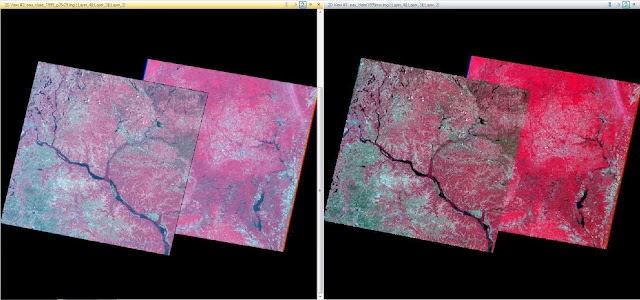
If you have a study area that is larger than the spatial extent of one satellite image, or is located on the intersection between two images, you will have to perform an mosaic to combine the two satellite scenes to that encase the entire study area. The first type of mosaic we will use is the Mosaic Express. For this type of mosaic, all you have to do is bring both images into the same viewer and use the Raster tool Mosaic Express. After the model is run, you get a resulting image that has combined the two satellite scenes into one. This method is not very effective for it leaves a clear indication that the two images were not originally together and have completely different color values, saturation, and even hue. This mosaic is located below in figure 3.
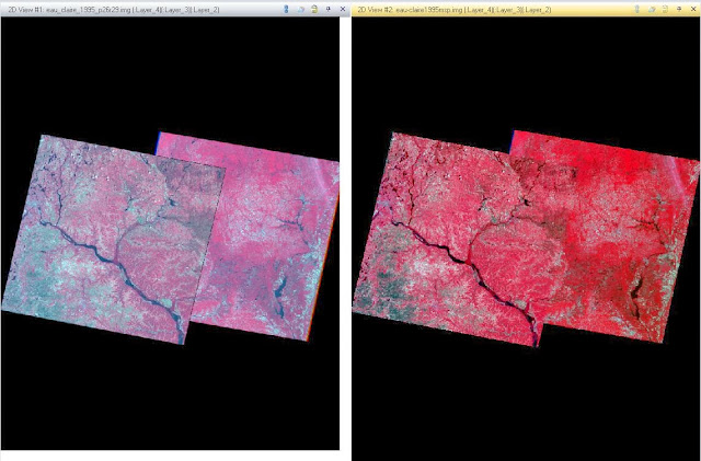
The more effective mosaic model we can run is called the Mosaic Pro. This is also a Raster tool and is run similar to the mosaic express but has a few more options we can customize. The main option we want to activate is a Color Correction tool called Use Histogram Matching. This will match the two image's histograms which will help blend them together. We are also going to us the Overlay tool  to incorporate the brightness values of the top image at the area of intersection. That will also help blend the two images together. After the model is run, the resulting image is shows a vastly improved scene in which the area of intersection is blended together with more accuracy than the Mosaic Express model. There are still some areas along the intersection where it is clearly visible that the two images were combined but it is a far more accurate mosaic than the Express. The Mosaic Pro images can be seen in Figure 4.

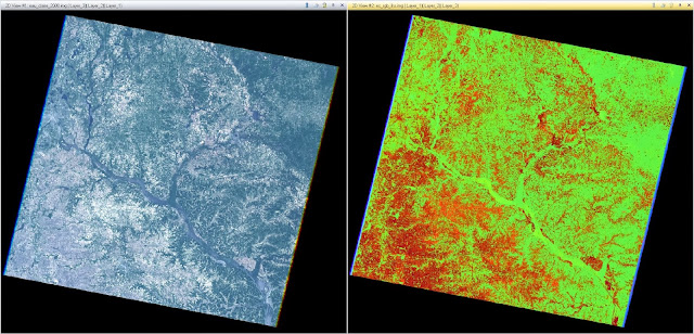
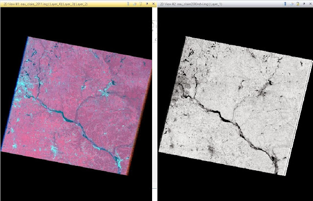
Another useful tool to help identify features in a satellite image is a Band Ratio method called normalized difference vegetation index, or NDVI. This is particularly useful to identify where green vegetation is located on a satellite image. NDVI is a Unsupervised Raster tool that uses the 'Landsat TM' sensor and NDVI function. Once you run the model, it transforms all green vegetation into a bright white color and everything else into a shade of gray. That makes it very easy to distinguish between vegetation and other features that are on the image. The result of the NDVI method can be seen in Figure 5 below.

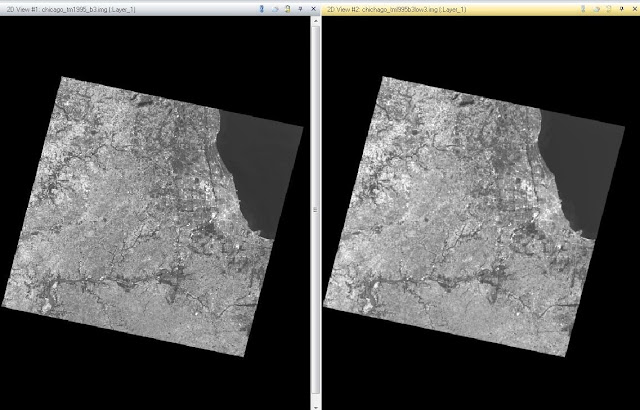
Now lets look at some Spatial Image enhancement techniques that can be applied to remotely sense images. The first technique is going to be applying a low pass filter on a high frequency image. The reason we want to do this low pass filter is because a high frequency image has significant changes in brightness values over short distances which can make the image features hard to distinguish. The filter we want to apply to our image is a 5x5 Low Pass Convolution filter, which can be found under the Raster Spatial tools. As you can see in Figure 6 below, the newly filtered image has less variation in brightness which blends the features together.
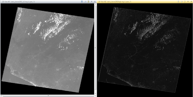
In turn, you can take a low frequency image and apply a high pass filter on it to sharpen up the features by having more variations of brightness values over a shorter distance. To do this, follow the same steps when using a low pass filter but instead of selecting 5x5 Low Pass Convolution, choose 5x5 High Pass Convolution. The resulted image has more depth in brightness values over shorted distances which gives more variation to different features that are located closely together. The transformation displaying the before and after can be seen in Figure 7.
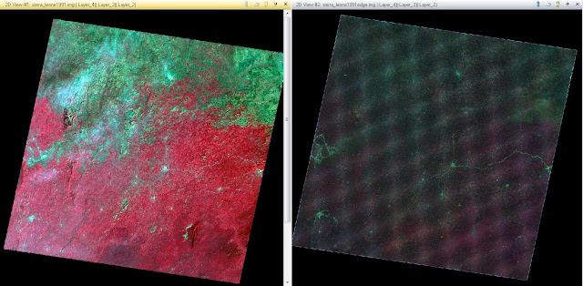
The last spatial technique we used in this lab is Edge enhancement, specifically, Laplacian Edge Detection. This is also a Convolution tool but instead of choosing a 5x5 filter, we are choosing a 3x3 Laplacian Edge Detection not with a Normalized Kernel. This method sharpens the image by locally increasing the contrast at discontinuities and gives it a more natural look. The result after the Laplacian convolution mask was applied can be seen in Figure 8 below.

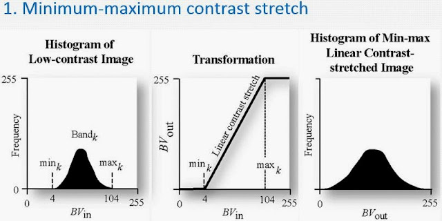
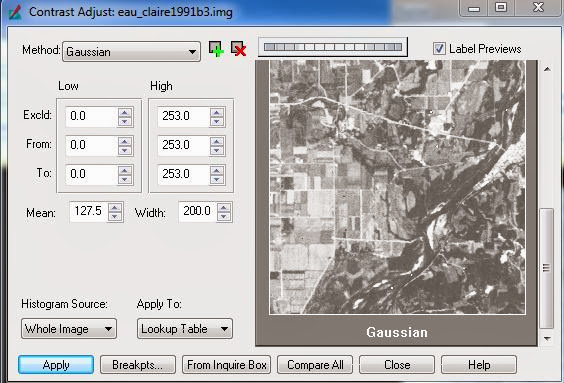
Now lets move onto some Spectral enhancement techniques. The first type of enhancement we applied to the satellite image is called the Minimum-Maximum contrast stretch. This is used with images that have a Gaussian histogram. The stretch uses the histogram and extends the minimum brightness value(BV) to 0 and the maximum BV to 255. An example of what the histogram looks like before and after a min-max stretch is in Figure 9. This technique is a Panchromatic General Contrast tool and needs to have the method type changed to Gaussian. That will show an area of the image and how it compares to other method types. Figure 10 shows the min-max contrast stretch on the Gaussian image.
Another Spectral enhancement technique we used on our satellite image was a technique called piecewise stretch. It is a General Contrast tool that allows us to specify the ranges we want the linear stretch to be applied on the histogram. We choose to have the Low range to be from 6 to 30, the Middle range from 31 to 76, and the High range from 77 to 109.The images in Figure 11 show the before and after effects of the Piecewise stretch.
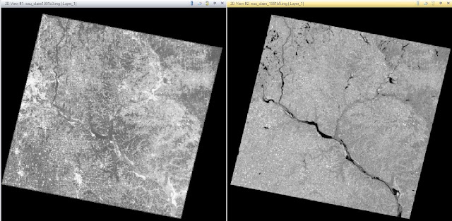
The last Spectral enhancement technique that was used on the satellite image was the Histogram Equalization. This nonlinear stretch redistributes pixel values in the image so the pixels in the output image are equally distributed among the range of output values. That results in a relatively flat histogram which in turn increases the contrast in the image. The original image, Figure 12 - left, has a low contrast with most of the color in the middle gray area with some white. Compared to the image on the right which has a higher contrast due to the histogram equalization that was applied to it. The technique is a Radiometric Raster tool that automatically redistributes the pixel values, resulting in a higher contrast image.

The last part of the lab involved Binary change detection or image differencing. In order to do this, you need two images to create the new output image. The Two Image Functions tool allows us to then use the Two Input Operators in which we input the two image files and name the output file that will be created. To simplify this process we only used one layer from both images, in this case we used layer 4. The resulting photo is located in Figure 13 below.
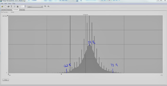
Now that we have the image that was created from subtracting the two primary satellite images, we can estimate the threshold of change-no-change. To figure out which areas actually changed, we can look at the histogram tails. To decide where the tails actually start we had to do a little math. The cut off point of the tails were decided with the equation mean + 1.5*standard deviation. The numbers we used for the tails can be seen in Figure 14.
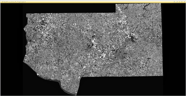
Now we can map out the changes that occurred within the image which was between August 1991 and August 2011. For this equation, we needed to use the Model Maker in Erdas Imagine 2013. By using the Function object between the two images, we ran the equation ($n1_ec_envs_2011_b4 - $n2_ec_envs_1991_b4 + 127) and this gave us our output file. The last calculating step comes next to determine the upper tail of the new histogram which contains the changed areas. For this we used mean + (3*standard deviation). Then, by using another Model Maker and the value we just calculated, we can finally get the pixels that changed between the two images. The Model Maker Functional Definition equation we used was: EITHER 1 IF ( $n1_ec_91> change/no change threshold value) OR 0 OTHERWISE. This means show all pixels with value above 'change/no change threshold value' and mask out those that are below the 'change/no change threshold value'. With the output file created, I opened it up into ArcMap and put an overlay image on it and changed the feature colors to get the resulting image in Figure 15.

Results

Figure 1 - RGB to IHS Transformation

Figure 2 - RGB to RGB Stretched Transformation

Figure 3 - Mosaic Express

Figure 4 - Mosaic Pro

Figure 5 -  Normalized Difference Vegetation Index (NDVI)

Figure 6 - 5x5 Low Pass Convolution

Figure 7 - 5x5 High Pass Convolution

Figure 8 - Laplacian Edge Detection

FIgure 9 - Minimum - Maximum Contrast Stretch

Figure 10 - Minimum - Max Contrast Stretch - Gaussian

Figure 11 - Piecewise Contrast

Figure 12 - Histogram Equalization

Figure 13 - Difference Image

Figure 14 - Histogram User-specified change/no change threshold

Figure 15 - Change in Pixel values in Eau Claire County and four other neighboring counties between August 1991 and August  2011.

Remote Sensing Lab 4: Miscellaneous image functions

Goal
This lab had five goals and techniques that would help us become familiar with image functions in Remote Sensing using Erdas 2011. The first goal is to understand how to take a study area (AOI) from a larger satellite image scene. The second goal is creating a high spatial resolution image from a low spatial resolution image to aid in visual interpretation. The third goal involves the use of radiometric enhancement techniques to improve image spectral and radiometric quality. The fourth goal involves linking Google Earth to images we have open in Erdas 2011 and use the classification data from Google Earth to aid in interpreting the image.
The last goal teaches us to re-size the pixels of an image to increase or decrease the file size.

Methods
Lets start off by selecting our study area (AOI) from a larger satellite image. We are going to be doing this using a Inquire Box which is located under the Raster tools. Then just move and re-size the Inquire Box to the AOI and apply the change. Now that we have our location set, we have to separate it from the larger image. To do that, use the tool Create Subset Image, insert the input/output options, and hit From Inquire Box. That will make sure the new image we removed from the large satellite image is the one we had highlighted with the inquire box. The original satellite image and the inquire box image can be seen below in Figure 1. You can also get an AOI out of a larger image by using a shape file. We used a shape file of counties and selected two that were on the satellite image. You then save the area as an .aoi file. This result can be seen below as Figure 2.

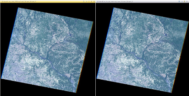
If you have a coarse resolution image and need it to have higher spatial resolution, you can Pan sharpen it. Pan sharpening optimizes image spatial resolutions to aid in visual interpretation. In our example, we used a 15 meter panchromatic image and a 30 meter reflective image to create a high resolution image. By using the Resolution Merge tool resulting image has 15x15 meter spatial resolution and the reflective properties of the second image. The results can be seen in Figure 3 below.

 Radiometric enhancement can be very useful when looking at a low quality satellite images that have been affected by distortion due to water vapor or other interference's . To correct that distortion, we can perform a Haze Reduction technique. In Figure 4 below, we can see the image on the left has haze distortion. To remove that, we can use a Radiometric tool called Haze Reduction. Once it is applied, the resulting image is haze free, which can be seen on the right image in Figure 4.

The next technique that we used in this lab was linking an image viewer to Google Earth. To get started, we had to open an image file in Erdas 2011 and use the Connect to Google Earth tool. That opens up a new viewer in which Google Earth uses to display the image. Then by clicking the Match GE to View tool, Google Earth matches the image you have displayed with the same spatial extent. This is helpful in the case you do not have much spatial information on your AOI and need to use Google Earths data to increase your knowledge base on the location. The synced up views can be seen in Figure 5 below.

The last technique used in this lab is Re-sampling. Re-sampling is the process of changing the pixel sizes in an image to reduce/increase file size and smoothness of images. Before we can re-size them, we need to know what the current pixel sizes are. To do that, to go the Image Metadata and look under the map information section. Once you have the pixel size, use the Raster tool: Spatial and Re-sample Pixel Size. We are using the Nearest Neighbor method and Bi-linear Interpolation methods to modify the new pixels, and changing the size from 30x30 meters, to 20x20. If you go back into the metadata for the image, you can see that the pixel size has been changed and the overall image is smoother. The only downside to having smaller pixels is that the file size is going to be larger. So make sure you have plenty of storage space. The re-sampled images can be seen below in Figure 6. The original image with 30x30 meter pixels is on the left, the 20x20 meter Nearest Neighbor re-sampled image in is the middle, and the 20x20 meter Bi-linear Interpolation image is on the right.

Results

Figure 1 - Image Subset using inquire Box

Figure 2 - Image Subset using Shape File

Figure 3 - Resolution Merge: Pan sharpen

Figure 4 - Haze Reduction

Figure 5 - Linking to Google Earth

Figure 6 - Re-sampling: Nearest Neighbor and Bi-linear Interpolation

US Dept. of State Geographer

2013 Google Image Landsat

http://www.google.com/earth/